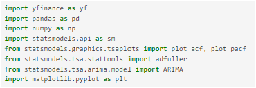
The below illustrates a simplified example on how forecasting can be performed on time-series data using ARIMA modelling. For this showcase we will be using the past 1 year historical data to forecast the price of gold futures.

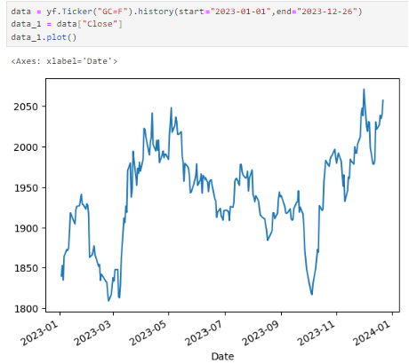
For this example, we will explore modelling of the gold futures price below.
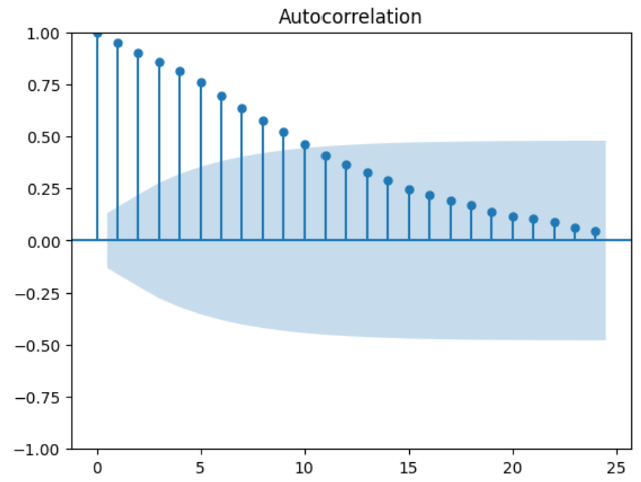
Next we will split the time series into training and test sets, 90% and remaining 10% respectively. After which we will look at the correlation of the time series with its lag through the ACF and PACF plots. Below, the PACF plot (right side) shows partial autocorrelation having a significant spike at lag 1 while in the ACF plot (left side), the correlations with the lags are positive and having a gradual decay.


In addition, we check to ensure data is stationary using Augmented Dickey-Fuller (ADF) test for the null hypothesis that there is a unit root (non-stationary). Given p-value < 5% significance level, we can reject the null hypothesis, so the ADF test suggests that our time series is likely to be stationary and we will not need to utilize differencing on the data.

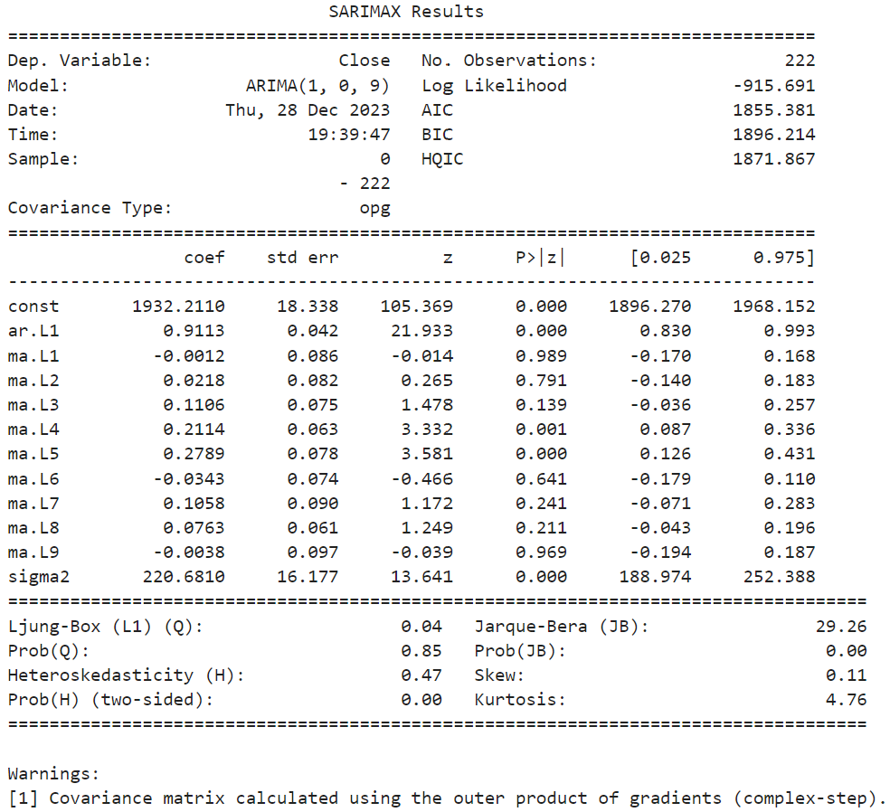
Since we will not be applying differencing (d=0), now we have to determine the other parameters (p,q) for the model we will be using from ARIMA (p,d,q). Given PACF plot having a significant spike at lag 1, while the ACF plot showed significant spikes up to lag 9, we will try p=1 and q=9. Next we will fit the ARIMA model using statsmodel package.

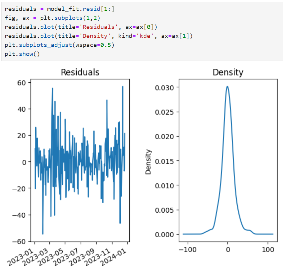
Before making predictions, the model needs to capture sufficient info from the data and the residuals should look like white noise. From the plots below, the residual seems random and density looks normally distributed with mean 0.
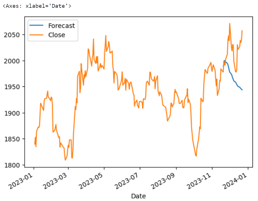
Next is to fit the model using the test set data (remaining 10%) and backtest the predictions against the actual series. As we see from the results below, time series predictions are difficult given the forecast was a downtrend while the actual closing price continued on the uptrend before a sharp retracement and then followed by another continuation of the uptrend.

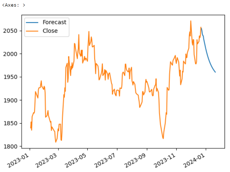
If we fit the entire dataset (train+test) to forecast the future prices, it appears that the gold price is also forecasted to retrace from its current values.

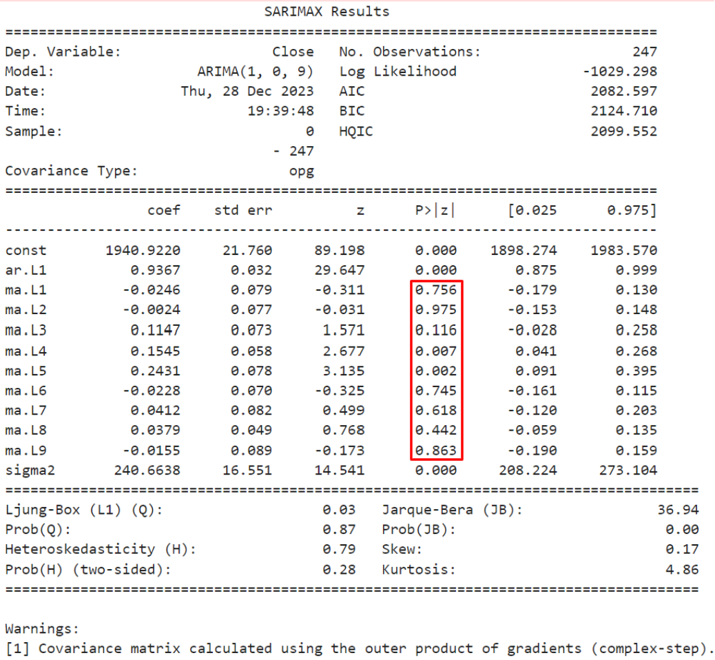

However from the previous model, most of the MA coefficients do not appear to be statistically significant (red highlight). Perhaps we can try excluding the MA and set different "q" paramaters for the model (p,d,q). In this case, we try setting "q" to 0.
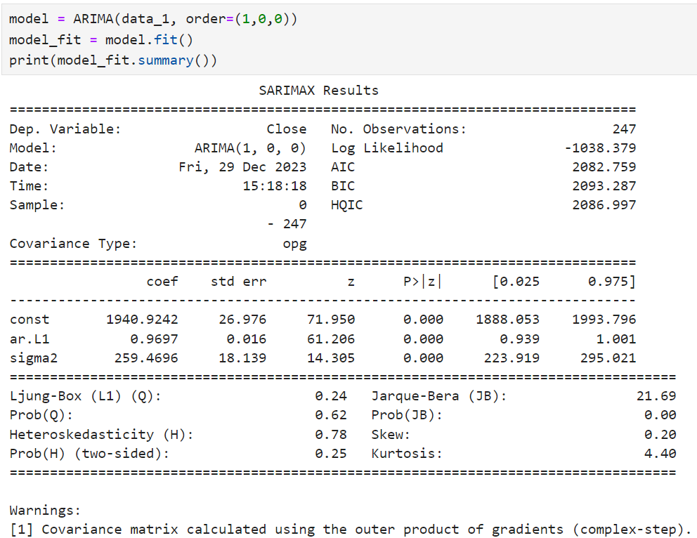
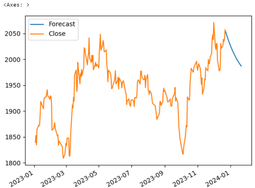
After adjusting, it appears the forecasted results still appear to predict a downtrend but shows a less steep retracement compared to the prior model. In conclusion, making time-series predictions is a challenging and iterative process and there are many variations we can tweak depending on the business context and nature of the objective.